Welcome to Part 2 of a beginners guide to AFL analytics and programming in R! This post will be following directly on from my first post, which you can access here. It covers the main points of installing R and RStudio and loading AFL data into your workspace.
If you have any questions during this tutorial, you can tweet at me @crow_data_sci. If you’ve got a useless stat, feel free to message at us Useless AFL Stats.
Starting a new script
Upon opening RStudio, check that you are in the right project. In the top left corner, there is a drop down menu, and choose the AFL_scripts project. The name might be named differently, or you can create a new project by following the top default options.
Now that we are in the right directory, create a new R script from the File -> New File -> R Script in the top left corner. You should now see the script open, and you can save it and name it accordingly.
Loading pacakges and AFL tables data
We are going to load in the 2020 AFL season from afltables using the fantastic fitzRoy package. Assuming you followed Part 1, these packages should already be installed. If not, use install.packages('dplyr') for a first time install for each package.
# setting the start data to 2020-01-01 only loads in 2020 data
afltables <- get_afltables_stats(start_date = '2020-01-01')
## Returning data from 2020-01-01 to 2020-10-27## Downloading data##
## Finished downloading data. Processing XMLs## Finished getting afltables data# clean up the column names
names(afltables) <- to_snake_case(names(afltables))Recap
From the previous post, we were introduced to the a couple of dplyr functions: select, group_by, summarise, mutate, filter and arrange. Let’s put them together to answer the following questions:
Q1. Which player averaged the highest contested possessions?
Q2. Which team per round had the highest ratio of kicks to handballs?
Q1. Which player averaged the highest contested possessions?
First step, select the columns we need. Records in afltables are at a player level, ie each row is a player.
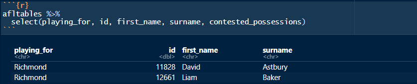
afltables %>%
  select(playing_for, id, first_name, surname, contested_possessions)
## # A tibble: 7,084 x 5
## playing_for id first_name surname contested_possessions
## <chr> <dbl> <chr> <chr> <dbl>
## 1 Richmond 11828 David Astbury 5
## 2 Richmond 12661 Liam Baker 10
## 3 Richmond 12535 Shai Bolton 3
## 4 Richmond 12456 Nathan Broad 1
## 5 Richmond 12010 Josh Caddy 2
## 6 Richmond 12431 Jason Castagna 0
## 7 Richmond 11666 Trent Cotchin 9
## 8 Richmond 11557 Shane Edwards 6
## 9 Richmond 12576 Jack Graham 4
## 10 Richmond 11879 Dylan Grimes 2
## # ... with 7,074 more rowsThe raw data looks good, so now we can group by each player to find out their average contested possessions. Remember to drop the grouping after the summarise function.
afltables %>%
  select(playing_for, id, first_name, surname, contested_possessions) %>%
  group_by(playing_for, id, first_name, surname) %>%
  summarise(
    avg_cont_pos = mean(contested_possessions),
    .groups = 'drop' # drop the grouping
  )
## # A tibble: 654 x 5
## playing_for id first_name surname avg_cont_pos
## <chr> <dbl> <chr> <chr> <dbl>
## 1 Adelaide 6623 Kyle Hartigan 3.67
## 2 Adelaide 11535 Bryce Gibbs 3.67
## 3 Adelaide 11634 David Mackay 4.5
## 4 Adelaide 11713 Taylor Walker 4.14
## 5 Adelaide 11792 Rory Sloane 8.42
## 6 Adelaide 11865 Tom Lynch 5
## 7 Adelaide 11891 Brodie Smith 4.25
## 8 Adelaide 11989 Daniel Talia 3.64
## 9 Adelaide 12035 Paul Seedsman 4.33
## 10 Adelaide 12106 Luke Brown 3.59
## # ... with 644 more rowsEach player now has their average, lets arrange the data in descending order (highest at the top).
afltables %>%
  select(playing_for, id, first_name, surname, contested_possessions) %>%
  group_by(playing_for, id, first_name, surname) %>%
  summarise(
    avg_cont_pos = mean(contested_possessions),
    .groups = 'drop' # drop the grouping
  ) %>%
  arrange(desc(avg_cont_pos))
## # A tibble: 654 x 5
## playing_for id first_name surname avg_cont_pos
## <chr> <dbl> <chr> <chr> <dbl>
## 1 Melbourne 12410 Clayton Oliver 13.4
## 2 Collingwood 12054 Adam Treloar 12.9
## 3 Melbourne 12430 Christian Petracca 12.7
## 4 Fremantle 11834 Nat Fyfe 12.5
## 5 Brisbane Lions 12055 Lachie Neale 12.5
## 6 Gold Coast 12533 Hugh Greenwood 12.4
## 7 Carlton 12261 Patrick Cripps 11.9
## 8 Western Bulldogs 11898 Tom Liberatore 11.4
## 9 Sydney 11953 Luke Parker 11.3
## 10 Geelong 11700 Patrick Dangerfield 11.2
## # ... with 644 more rowsLet’s make a small adjustment to the summarise, adding in the amount of games played this season, and we can also add in another stat, for example average handballs per game (which we are going to arrange by).
afltables %>%
  select(playing_for, id, first_name, surname, contested_possessions, handballs) %>%
  group_by(playing_for, id, first_name, surname) %>%
  summarise(
    avg_cont_pos = mean(contested_possessions),
    avg_handballs = mean(handballs),
    n = n(), #n() counts the amount of rows in this group
    .groups = 'drop' # drop the grouping
  ) %>%
  arrange(desc(avg_handballs)) %>%
  select(-id) # a '-' in before a column drops it
## # A tibble: 654 x 6
## playing_for first_name surname avg_cont_pos avg_handballs n
## <chr> <chr> <chr> <dbl> <dbl> <int>
## 1 Adelaide Matt Crouch 9.69 16 16
## 2 Hawthorn Tom Mitchell 10.4 15.1 17
## 3 Western Bulldogs Jack Macrae 10.3 14.9 18
## 4 Collingwood Adam Treloar 12.9 14.7 10
## 5 Brisbane Lions Lachie Neale 12.5 13.8 19
## 6 Melbourne Clayton Oliver 13.4 13.5 17
## 7 Collingwood Brayden Sier 7.33 12.7 3
## 8 Essendon Zach Merrett 7.75 12.4 16
## 9 Fremantle Nat Fyfe 12.5 12.1 14
## 10 Adelaide Rory Laird 8.82 11.9 17
## # ... with 644 more rowsInteresting to note that Collingwood’s Brayden Sier played 3 games averaging over 12 handballs, so maybe we want to filter out players with a low amount of games.
afltables %>%
  select(playing_for, id, first_name, surname, contested_possessions, handballs) %>%
  group_by(playing_for, id, first_name, surname) %>%
  summarise(
    avg_cont_pos = mean(contested_possessions),
    avg_handballs = mean(handballs),
    n = n(), #n() counts the amount of rows in this group
    .groups = 'drop' # drop the grouping
  ) %>%
  filter(n > 10) %>% #games greater than 10
  arrange(desc(avg_handballs)) %>%
  select(-id) # a '-' in before a column drops it
## # A tibble: 348 x 6
## playing_for first_name surname avg_cont_pos avg_handballs n
## <chr> <chr> <chr> <dbl> <dbl> <int>
## 1 Adelaide Matt Crouch 9.69 16 16
## 2 Hawthorn Tom Mitchell 10.4 15.1 17
## 3 Western Bulldogs Jack Macrae 10.3 14.9 18
## 4 Brisbane Lions Lachie Neale 12.5 13.8 19
## 5 Melbourne Clayton Oliver 13.4 13.5 17
## 6 Essendon Zach Merrett 7.75 12.4 16
## 7 Fremantle Nat Fyfe 12.5 12.1 14
## 8 Adelaide Rory Laird 8.82 11.9 17
## 9 Collingwood Scott Pendlebury 9.6 11.9 15
## 10 Melbourne Christian Petracca 12.7 11.7 17
## # ... with 338 more rowsAdding %>% View() to the end of the pipeline brings up an interactive spreadsheet, very useful for interacting with the data.
Q2. Which team per round had the highest ratio of kicks to handballs?
Using the same process as before, but we now need to group by 2 columns, round and playing_for. We are going to sum the handballs and kicks for each game.
afltables %>%
  select(round, playing_for, kicks, handballs) %>%
  group_by(round, playing_for) %>%
  summarise(
    s_kicks = sum(kicks),
    s_hball = sum(handballs),
    .groups = 'drop'
  )
## # A tibble: 322 x 4
## round playing_for s_kicks s_hball
## <chr> <chr> <dbl> <dbl>
## 1 1 Adelaide 142 108
## 2 1 Brisbane Lions 185 103
## 3 1 Carlton 188 114
## 4 1 Collingwood 191 161
## 5 1 Essendon 192 147
## 6 1 Fremantle 166 120
## 7 1 Geelong 176 98
## 8 1 Gold Coast 173 123
## 9 1 Greater Western Sydney 167 91
## 10 1 Hawthorn 187 111
## # ... with 312 more rowsWe have the total kicks and handballs for each team in each round, and we can use mutate to perform a calculation.
afltables %>%
  select(round, playing_for, kicks, handballs) %>%
  group_by(round, playing_for) %>%
  summarise(
    s_kicks = sum(kicks),
    s_hball = sum(handballs),
    .groups = 'drop'
  ) %>%
  mutate(ratio = s_kicks/s_hball*100) %>%
  arrange(ratio)
## # A tibble: 322 x 5
## round playing_for s_kicks s_hball ratio
## <chr> <chr> <dbl> <dbl> <dbl>
## 1 2 Western Bulldogs 142 177 80.2
## 2 18 North Melbourne 164 196 83.7
## 3 14 Essendon 151 174 86.8
## 4 4 Richmond 149 164 90.9
## 5 16 Western Bulldogs 157 162 96.9
## 6 15 Adelaide 159 161 98.8
## 7 5 Western Bulldogs 166 165 101.
## 8 9 Western Bulldogs 141 137 103.
## 9 14 Port Adelaide 163 158 103.
## 10 9 Melbourne 150 145 103.
## # ... with 312 more rowsYou can add %>% View to view the data interactively. I’d also recommend using the filter button to further sort your data.
Calculating Home vs Away and wins
The data that we import into R doesn’t record whether the players were Home or Away, or if the result was a draw or loss. We are going to add these in using mutate and case_when, a powerful tool that allows multiple if_else statements.
Home vs Away
We are going to create a new column named h_a. afltables provides a column with the home team’s name, and another column of the team the player is playing for, and we can use this with a bit of logic in an if_else statement.
afltables %>%
  select(playing_for, id, first_name, surname, home_team, away_team) %>%
  mutate(
    h_a = if_else(playing_for == home_team, 'H', 'A')
  )
## # A tibble: 7,084 x 7
## playing_for id first_name surname home_team away_team h_a
## <chr> <dbl> <chr> <chr> <chr> <chr> <chr>
## 1 Richmond 11828 David Astbury Richmond Carlton H
## 2 Richmond 12661 Liam Baker Richmond Carlton H
## 3 Richmond 12535 Shai Bolton Richmond Carlton H
## 4 Richmond 12456 Nathan Broad Richmond Carlton H
## 5 Richmond 12010 Josh Caddy Richmond Carlton H
## 6 Richmond 12431 Jason Castagna Richmond Carlton H
## 7 Richmond 11666 Trent Cotchin Richmond Carlton H
## 8 Richmond 11557 Shane Edwards Richmond Carlton H
## 9 Richmond 12576 Jack Graham Richmond Carlton H
## 10 Richmond 11879 Dylan Grimes Richmond Carlton H
## # ... with 7,074 more rowsWins and Losses
In order to calculate whether there was a win or loss, we need to do something similar. afltables has home team and home score which we can use to reverse engineer a win loss column. Creating a new column w_l using a dplyr function, case_when
afltables %>%
  select(id, first_name, surname, playing_for, home_team, away_team, home_score, away_score) %>%
  mutate(
    w_l = case_when(
      playing_for == home_team & home_score > away_score ~ 'W',
      playing_for == home_team & home_score < away_score ~ 'L',
      playing_for == away_team & away_score > home_score ~ 'W',
      playing_for == away_team & away_score < home_score ~ 'L',
      TRUE ~ 'D'
    )
  ) # %>% View()
## # A tibble: 7,084 x 9
## id first_name surname playing_for home_team away_team home_score
## <dbl> <chr> <chr> <chr> <chr> <chr> <int>
## 1 11828 David Astbury Richmond Richmond Carlton 105
## 2 12661 Liam Baker Richmond Richmond Carlton 105
## 3 12535 Shai Bolton Richmond Richmond Carlton 105
## 4 12456 Nathan Broad Richmond Richmond Carlton 105
## 5 12010 Josh Caddy Richmond Richmond Carlton 105
## 6 12431 Jason Castag~ Richmond Richmond Carlton 105
## 7 11666 Trent Cotchin Richmond Richmond Carlton 105
## 8 11557 Shane Edwards Richmond Richmond Carlton 105
## 9 12576 Jack Graham Richmond Richmond Carlton 105
## 10 11879 Dylan Grimes Richmond Richmond Carlton 105
## # ... with 7,074 more rows, and 2 more variables: away_score <int>, w_l <chr>Translated to English
- IF playing for is the same as the home team AND home score is greater than away score THEN it’s a win ELSE
- IF playing for is the same as the home team AND home score is less than away score THEN it’s a win ELSE
- IF playing for is the same as the away team AND home score is greater than away score THEN it’s a win ELSE
- IF playing for is the same as the away team AND home score is less than away score THEN it’s a win ELSE
- Its a draw
All together now
This type of calculation should be completed when you first load in the data, which might look something like this.
# setting the start data to 2020-01-01 only loads in 2020 data
afltables <- get_afltables_stats(start_date = '2020-01-01')
## Returning data from 2020-01-01 to 2020-10-27## Downloading data##
## Finished downloading data. Processing XMLs## Finished getting afltables data# clean up the column names
names(afltables) <- to_snake_case(names(afltables))
# create a new dataset with a combined mutate function
afltables_new <- afltables %>%
mutate(
h_a = if_else(playing_for == home_team, 'H', 'A'),
w_l = case_when(
playing_for == home_team & home_score > away_score ~ 'W',
playing_for == home_team & home_score < away_score ~ 'L',
playing_for == away_team & away_score > home_score ~ 'W',
playing_for == away_team & away_score < home_score ~ 'L',
TRUE ~ 'D'
)
)
#View(afltables_new)This allows for more in depth analysis, as you can now filter out losses, group by wins, and compare away to home performances. Here’s a basic example: Who had the most losses this season?
afltables_new %>%
  group_by(playing_for, id, first_name, surname, w_l) %>%
  count() %>%
  filter(w_l == 'L') %>%
  arrange(desc(n))
## # A tibble: 628 x 6
## # Groups: playing_for, id, first_name, surname, w_l [628]
## playing_for id first_name surname w_l n
## <chr> <dbl> <chr> <chr> <chr> <int>
## 1 Adelaide 12106 Luke Brown L 14
## 2 Adelaide 12165 Rory Laird L 14
## 3 Adelaide 12473 Reilly OBrien L 14
## 4 North Melbourne 4180 Shaun Higgins L 14
## 5 North Melbourne 11686 Todd Goldstein L 14
## 6 North Melbourne 11902 Shaun Atley L 14
## 7 North Melbourne 12109 Josh Walker L 14
## 8 North Melbourne 12246 Luke McDonald L 14
## 9 North Melbourne 12343 Trent Dumont L 14
## 10 North Melbourne 12502 Jy Simpkin L 14
## # ... with 618 more rowsConclusion
Thanks for completing this tutorial, you can check out the script I used to generate this analysis here. You can ask me questions about the tutorial at my twitter @crow_data_sci. My DM’s are always open!
Next tutorial will be on the topic of ggplot, R’s plotting and charting tools, and we’ll be creating some pretty cool charts!