The data

Here’s some data I prepared earlier, 17 venues with corresponding latitude and longitude. These are Australian based venues that have been used in the last 3 years of the AFL regular season.

library(dplyr)
library(tidyr)
afl_venue_locations <- read.csv("post_data/afl_venue_locations.csv")

library(leaflet)

leaflet(data = afl_venue_locations) %>% addTiles() %>%
  addMarkers(~longitude, ~latitude, popup = ~venue, label = ~venue)

Given these 17 locations, and we want to find the shortest path that allows us to visit each of the grounds and finish where we started. To start off we need a distance matrix, a calculation of the distance between each venue. We are going to use the geosphere package with built in functions to calculate distances from the venues’ latitude and longitude coordinates.

The data prep

library(geosphere)

afl_venue_coords <- afl_venue_locations %>% select(longitude, latitude)

distance_matrix <- as.matrix(
  distm(afl_venue_coords, fun = distHaversine)
)/1000 #convert metres to kilometres

rownames(distance_matrix) <- afl_venue_locations$venue
colnames(distance_matrix) <- afl_venue_locations$venue

Our distance matrix has been computed. You’ll notice that the diagonals are all 0, which makes sense given its the same location. Also the matrix is symmetrical along the diagonal: Walking from the MCG to Docklands is the same as the return journey. Please note that this is a “As the crow flies” implementation, a straight line from venue to venue.

Model Building

I chose to use the ompr implementation of the TSP, which I found to be pretty stable and quick*. We will also need the development version of ompr to get access to the vectorised version of the algorithm.

*I haven’t tried any others.

install.packages("ompr")
devtools::install_github("dirkschumacher/ompr.roi") #or cran version higher than 0.8.0.9
install.packages("ROI.plugin.glpk")

library(ompr)
#specify the dimensions of the distance matrix
n <- length(afl_venue_locations$id)

#create a distance extraction function
dist_fun <- function(i, j) {
    vapply(seq_along(i), function(k) distance_matrix[i[k], j[k]], numeric(1L))
}

model <- MILPModel() %>%
    # we create a variable that is 1 iff we travel from city i to j
    add_variable(x[i, j], i = 1:n, j = 1:n, 
                 type = "integer", lb = 0, ub = 1) %>%
    
    # a helper variable for the MTZ formulation of the tsp
    add_variable(u[i], i = 1:n, lb = 1, ub = n) %>% 
    
    # minimize travel distance
    set_objective(sum_expr(colwise(dist_fun(i, j)) * x[i, j], i = 1:n, j = 1:n), "min") %>%
    
    # you cannot go to the same city
    set_bounds(x[i, i], ub = 0, i = 1:n) %>%
    
    # leave each city
    add_constraint(sum_expr(x[i, j], j = 1:n) == 1, i = 1:n) %>%
    
    # visit each city
    add_constraint(sum_expr(x[i, j], i = 1:n) == 1, j = 1:n) %>%
    
    # ensure no subtours (arc constraints)
    add_constraint(u[i] >= 2, i = 2:n) %>% 
    add_constraint(u[i] - u[j] + 1 <= (n - 1) * (1 - x[i, j]), i = 2:n, j = 2:n)
model

## Mixed integer linear optimization problem
## Variables:
##   Continuous: 17 
##   Integer: 289 
##   Binary: 0 
## Model sense: minimize 
## Constraints: 306

The model has been built, now lets solve it.

#Solving the model

library(ompr.roi)
library(ROI.plugin.glpk)

result <- solve_model(model, with_ROI(solver = "glpk", verbose = TRUE))

## <SOLVER MSG>  ----
## GLPK Simplex Optimizer, v4.47
## 306 rows, 306 columns, 1330 non-zeros
##       0: obj =  0.000000000e+000  infeas = 5.000e+001 (34)
## *    54: obj =  2.453647438e+004  infeas = 0.000e+000 (1)
## *   128: obj =  8.936395032e+003  infeas = 0.000e+000 (1)
## OPTIMAL SOLUTION FOUND
## GLPK Integer Optimizer, v4.47
## 306 rows, 306 columns, 1330 non-zeros
## 289 integer variables, 272 of which are binary
## Integer optimization begins...
## +   128: mip =     not found yet >=              -inf        (1; 0)
## +   877: >>>>>  1.603882389e+004 >=  9.723428934e+003  39.4% (82; 1)
## +  1144: >>>>>  1.507632658e+004 >=  9.723917868e+003  35.5% (109; 5)
## +  2068: >>>>>  1.507157320e+004 >=  1.051733544e+004  30.2% (158; 31)
## +  2215: >>>>>  1.167150030e+004 >=  1.069026063e+004   8.4% (163; 32)
## +  3581: >>>>>  1.166830513e+004 >=  1.160505429e+004   0.5% (11; 353)
## +  3671: mip =  1.166830513e+004 >=     tree is empty   0.0% (0; 399)
## INTEGER OPTIMAL SOLUTION FOUND
## <!SOLVER MSG> ----

result_val <- round(objective_value(result), 2)
result_val

## [1] 11668.31

Nice! The shortest distance travelled to visit all venues is 11668km.

Results

How does this route look on a map?

solution <- get_solution(result, x[i, j]) %>% 
    filter(value > 0)

paths <- select(solution, i, j) %>% 
    rename(from = i, to = j) %>% 
    mutate(trip_id = row_number()) %>% 
    inner_join(afl_venue_locations, by = c("from" = "id"))

paths_leaflet <- paths[1,]
paths_row <- paths[1,]

for (i in 1:n) {
    paths_row <- paths %>% filter(from == paths_row$to[1])
    
    paths_leaflet <- rbind(paths_leaflet, paths_row)
}

leaflet() %>% 
    addTiles() %>%
    addMarkers(data = afl_venue_locations, ~longitude, ~latitude, popup = ~venue, label = ~venue) %>% 
    addPolylines(data = paths_leaflet, ~longitude, ~latitude, weight = 2)

Seems pretty intuitive, essentially a big loop around Australia.

model_max <- MILPModel() %>%
    # we create a variable that is 1 iff we travel from city i to j
    add_variable(x[i, j], i = 1:n, j = 1:n, 
                 type = "integer", lb = 0, ub = 1) %>%
    
    # a helper variable for the MTZ formulation of the tsp
    add_variable(u[i], i = 1:n, lb = 1, ub = n) %>% 
    
    # maximise travel distance
    set_objective(sum_expr(colwise(dist_fun(i, j)) * x[i, j], i = 1:n, j = 1:n), "max") %>%
    
    # you cannot go to the same city
    set_bounds(x[i, i], ub = 0, i = 1:n) %>%
    
    # leave each city
    add_constraint(sum_expr(x[i, j], j = 1:n) == 1, i = 1:n) %>%
    
    # visit each city
    add_constraint(sum_expr(x[i, j], i = 1:n) == 1, j = 1:n) %>%
    
    # ensure no subtours (arc constraints)
    add_constraint(u[i] >= 2, i = 2:n) %>% 
    add_constraint(u[i] - u[j] + 1 <= (n - 1) * (1 - x[i, j]), i = 2:n, j = 2:n)
model_max

## Mixed integer linear optimization problem
## Variables:
##   Continuous: 17 
##   Integer: 289 
##   Binary: 0 
## Model sense: maximize 
## Constraints: 306

result_max <- solve_model(model_max, with_ROI(solver = "glpk", verbose = TRUE))

## <SOLVER MSG>  ----
## GLPK Simplex Optimizer, v4.47
## 306 rows, 306 columns, 1330 non-zeros
##       0: obj =  0.000000000e+000  infeas = 5.000e+001 (34)
## *    54: obj =  2.453647438e+004  infeas = 0.000e+000 (1)
## *   166: obj =  3.605414246e+004  infeas = 0.000e+000 (1)
## OPTIMAL SOLUTION FOUND
## GLPK Integer Optimizer, v4.47
## 306 rows, 306 columns, 1330 non-zeros
## 289 integer variables, 272 of which are binary
## Integer optimization begins...
## +   166: mip =     not found yet <=              +inf        (1; 0)
## +   181: >>>>>  3.605414246e+004 <=  3.605414246e+004 < 0.1% (2; 0)
## +   181: mip =  3.605414246e+004 <=     tree is empty   0.0% (0; 3)
## INTEGER OPTIMAL SOLUTION FOUND
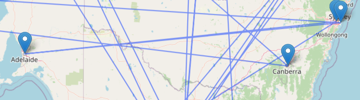
## <!SOLVER MSG> ----

result_val_max <- round(objective_value(result_max))

paste0('Total distance: ',result_val_max,'km')

## [1] "Total distance: 36054km"

solution_max <- get_solution(result_max, x[i, j]) %>% 
    filter(value > 0)

paths_max <- select(solution_max, i, j) %>% 
    rename(from = i, to = j) %>% 
    mutate(trip_id = row_number()) %>% 
    inner_join(afl_venue_locations, by = c("from" = "id"))

paths_max_leaflet <- paths_max[1,]
paths_max_row <- paths_max[1,]

for (i in 1:n) {
    paths_max_row <- paths_max %>% filter(from == paths_max_row$to[1])
    
    paths_max_leaflet <- rbind(paths_max_leaflet, paths_max_row)
}

leaflet() %>% 
    addTiles() %>%
    addMarkers(data = afl_venue_locations, ~longitude, ~latitude, popup = ~venue, label = ~venue) %>% 
    addPolylines(data = paths_max_leaflet, ~longitude, ~latitude, weight = 2)

Conclusion

Thanks for making it this far, you can check out the script I used to generate this analysis here. You can ask me questions about analysis at my twitter @crow_data_sci.

Make sure to check out ompr on github and follow the creator of this package on twitter, @dirk_sch.