Hypothetical Situation:
Fantasy points (FP) are a black box algorithm: no one knows what calculations are made to generate points. It’s a closely guarded industry secret and they don’t want to release their methodology to the rest of the AFL analytics community. We work for a rival ratings company and have been tasked with reverse engineering their methods, finding out what values are assigned to specific stats.
After a bit of corporate espionage, we now know the following:
- There are at most 13 stats in generating FP
- Kicks, handballs, marks, tackles, inside 50’s, bounces, frees for, frees against, one percenters, hitouts, goals, behinds & goal assists
- We are going to have to figure out which stats are used in calculations
- A small amount of random noise is added to further obscure the methodology
- We can assume that the noise is normally distributed
- A small percent of players have a chunk points randomly added or removed from the final score
- Further masks the methodology
- A shift may have been applied
- All data points have been increase or decreased by a fixed amount
- We also assume that each player, team and game a scored using the same methodology
We have been given the following data from the 2019 season with their corresponding FP:
See data generation:
library(dplyr)##
## Attaching package: 'dplyr'## The following objects are masked from 'package:stats':
##
## filter, lag## The following objects are masked from 'package:base':
##
## intersect, setdiff, setequal, union# afltables <- fitzRoy::get_afltables_stats(start_date = "2019-01-01", end_date = "2020-01-01") %>%
# rename_with(snakecase::to_snake_case)
# saveRDS(afltables, file = "reverse_eng_aftables.rds")
afltables <- readRDS("reverse_eng_aftables.rds")
set.seed(20120805)
afltables_2019_fp <- afltables %>%
select(kicks, handballs, marks, tackles, inside_50_s, bounces,
frees_for, frees_against, one_percenters, hit_outs, goals, behinds, goal_assists) %>%
mutate(
fp = kicks*3 + handballs*2 + marks*3 + tackles*4 + frees_for*1 +
frees_against*-3 + hit_outs + goals*6 + behinds, .before = 'kicks'
) %>%
rowwise() %>%
mutate(
fp = fp + 2,
fp = fp + rnorm(1, 0, 3), #mean of 0 and SD of 3
# fp = fp + rpois(1, 2),
# fp = fp + rgamma(1, 2),
# fp = fp + runif(1, -2, 2),
fp =
case_when(
runif(1) < 0.001 ~ fp + 20,
runif(1) > 0.999 ~ fp - 20,
T ~ fp
)
) %>% ungroup()print(afltables_2019_fp, width = Inf)## # A tibble: 9,108 x 14
## fp kicks handballs marks tackles inside_50_s bounces frees_for
## <dbl> <dbl> <dbl> <dbl> <dbl> <dbl> <dbl> <dbl>
## 1 101. 10 22 1 6 2 1 3
## 2 82.2 9 13 5 5 5 0 1
## 3 43.7 10 2 1 1 2 0 0
## 4 114. 13 12 12 3 3 0 1
## 5 64.5 8 13 3 2 3 0 1
## 6 27.1 4 1 2 1 0 0 1
## 7 81.4 14 8 2 6 3 0 1
## 8 57.3 8 1 3 4 0 0 0
## 9 47.3 5 6 2 3 1 0 0
## 10 56.6 4 4 3 5 0 0 3
## frees_against one_percenters hit_outs goals behinds goal_assists
## <dbl> <dbl> <dbl> <dbl> <dbl> <dbl>
## 1 1 0 0 0 0 0
## 2 2 0 0 0 0 1
## 3 2 0 0 1 0 0
## 4 0 1 0 0 1 1
## 5 1 1 0 0 1 0
## 6 1 0 0 1 0 0
## 7 4 3 0 1 1 1
## 8 0 2 0 0 0 0
## 9 1 2 0 0 1 0
## 10 1 7 0 0 0 0
## # ... with 9,098 more rowsWe want to investigate the effect of stats on the final result, and we are going to be using generalised linear models (GLMs).
Data exploration
A good place to start is a pair-wise correlation plot, which shows us predictive variables that may be highly correlated with each other. High correlation among predictors (multicollinearity) means you can predict one variable using another predictor variable and means we have redundancy in our data. This results in unstable parameter estimates of regression which makes it very difficult to assess the effect of independent variables on dependent variables. The standard error (SE) of such parameters becomes very high.
library(GGally)
ggcorr(afltables_2019_fp[,-1], geom = 'tile', layout.exp = 1,
       palette = "PuOr", hjust = 0.85, size = 3.5, label = T)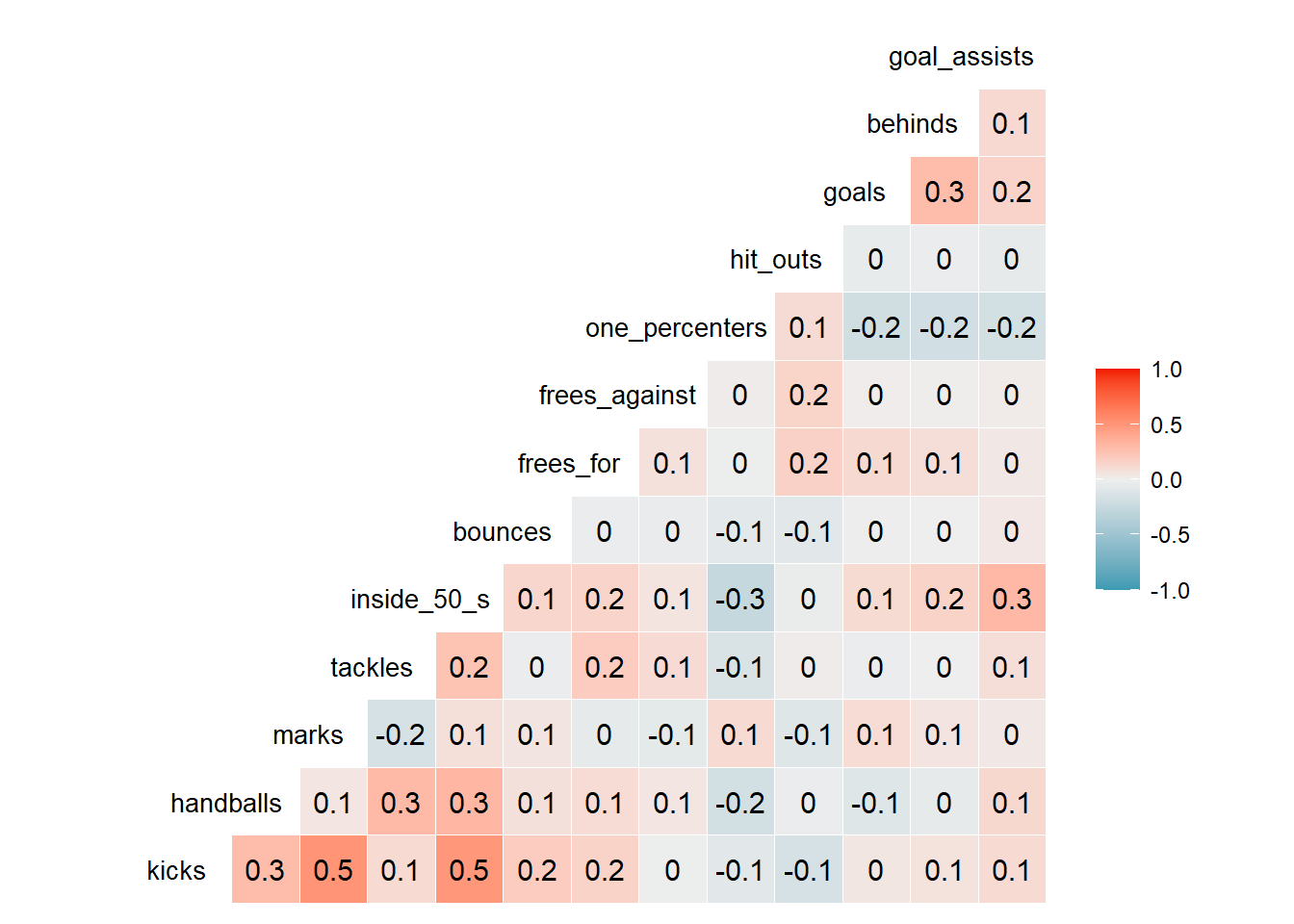
A correlation coefficient higher than 0.7 or lower than -0.7 is normally a cause for concern and would result in the removal of one of the variables (among other methods). In our data, the highest is 0.5 and we can now assume there is no multicollinearity between predictors.
Frequentist: Generalised Linear Models
Setting up the Formula
Formulas in R are set up with the following syntax: <response> ~ <variable1> + <variable2> + .... The response in this case is fp and variables (or predictors) are the stats.
In this example we won’t be investigating higher order interactions between terms.
formula <- "fp ~ kicks + handballs + marks + tackles + inside_50_s + bounces + frees_for +
frees_against + one_percenters + hit_outs + goals + behinds + goal_assists"
Choosing a (Distribution) Family
Next step in setting up a glm is to specify the distribution family, and a good way to choose one is to find out what domain the response exists in. This requires some knowledge of the data set and using a density plot can aid us in making a decision. Common distributions include:
- Gaussian (normal): Continuous unbounded (positive and negative real numbers)
- Gamma: Continuous positive
- Poisson: Integer positive
- Logistic: Continuous between 0 and 1 (or exclusively 0 and 1)
library(ggplot2)
ggplot(afltables_2019_fp, aes(x = fp)) +
  geom_density() +
  geom_rug() +
  ggtitle("Distribution of Fantasy Points") + ylab("") + xlab("FP")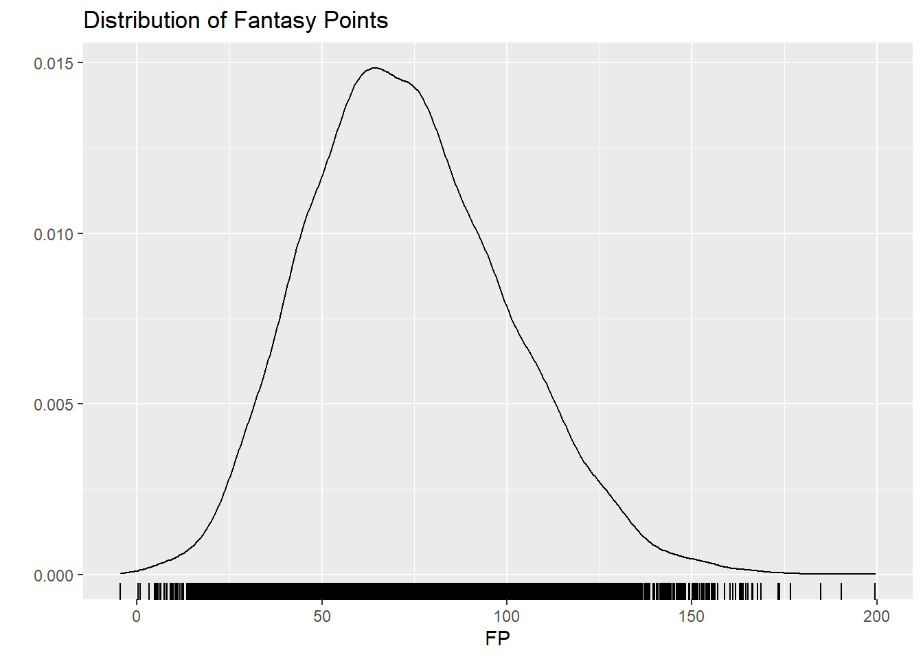
It’s important to note that FP can be negative, therefore FP is continuous and unbounded. With this knowledge, it makes sense to choose the normal (Gaussian) distribution.
Selecting a Link
We also need to select a link, and have 3 options with the Gaussian family:
- Identity: An increase in a stat corresponds to an linear increase in FP
- Log: An increase in a stat corresponds to an proportional increase in FP
- Inverse: An increase in a stat corresponds to an inverse increase in FP
We are going to be using the identity link, mainly because it’s the easiest to interpret and falls in line with standard linear regressions.
Running the Model + Interpretation
Putting it all together, and we can check the model summary.
glm1 <- glm(
  formula = formula,
  data = afltables_2019_fp,
  family = gaussian(link = "identity")
)

summary(glm1)
##
## Call:
## glm(formula = formula, family = gaussian(link = "identity"),
## data = afltables_2019_fp)
##
## Deviance Residuals:
## Min 1Q Median 3Q Max
## -23.8761 -2.0752 0.0152 2.0318 25.9347
##
## Coefficients:
## Estimate Std. Error t value Pr(>|t|)
## (Intercept) 2.0892003 0.1099437 19.002 <2e-16 ***
## kicks 3.0123931 0.0100210 300.608 <2e-16 ***
## handballs 1.9856901 0.0084920 233.830 <2e-16 ***
## marks 2.9898337 0.0164047 182.254 <2e-16 ***
## tackles 4.0360824 0.0161849 249.373 <2e-16 ***
## inside_50_s -0.0506948 0.0217571 -2.330 0.0198 *
## bounces 0.0411818 0.0462881 0.890 0.3737
## frees_for 0.9838578 0.0349754 28.130 <2e-16 ***
## frees_against -3.0309144 0.0337349 -89.845 <2e-16 ***
## one_percenters 0.0000577 0.0147666 0.004 0.9969
## hit_outs 0.9948819 0.0049551 200.778 <2e-16 ***
## goals 6.0652085 0.0381539 158.967 <2e-16 ***
## behinds 0.9645699 0.0491625 19.620 <2e-16 ***
## goal_assists -0.0034078 0.0537769 -0.063 0.9495
## ---
## Signif. codes: 0 '***' 0.001 '**' 0.01 '*' 0.05 '.' 0.1 ' ' 1
##
## (Dispersion parameter for gaussian family taken to be 9.806355)
##
## Null deviance: 6561783 on 9107 degrees of freedom
## Residual deviance: 89179 on 9094 degrees of freedom
## AIC: 46657
##
## Number of Fisher Scoring iterations: 2The model has been run and the results are being displayed above. Let’s examine it one step at a time.
Call shows us what model has been run. Deviance Residuals give a quick insight into the distribution of the residuals, which should be normally distributed around 0. Looks good so far, median \(\approx\) 0, and the quartiles and min/max are approximately symmetrical. We’ll be generating residuals plots to better understand it later.
Coefficients contains the information regarding estimates for the intercept and each stat. The estimate column (when using the “identity” link) shows the mean effect of each term in the model. For example, an increase by one (unit of) tackle increases FP by an estimate of 4.03.
Std. Error is the error term associated with the term’s estimate. Low standard error means the model in more certain that the mean estimate. The Pr(>|t|) is the p-value, a calculation based off the t-value and the degrees of freedom in the model.
The p-value is a uniquely frequentist form of test set up to determine whether the estimated mean has a statistically significant difference to 0 in the form of a null hypothesis. It can be described by following equation:
\[ H_0:\mu = 0 \]
where \(\mu\) is the term (variable). Normally a p-value of 0.05 is tested against, with a p-value greater than 0.05 meaning we “Accept the null hypothesis” (that the estimate is equal to 0, therefore has no effect). If the p-value is less than 0.05, then we “Fail to reject the null hypothesis” (that the estimate is not equal to 0, and has an effect).
(Intercept) has an estimate of 2.09, and is statistically significant (2e-16 is less than 0.05). We can use the Std. Error (Standard Error (SE)) to calculate a confidence interval, which is much easier to interpret (we use the constant 1.96 due to using a 95%CI, a 99%CI would use 2.58):
\[ 95\% \texttt{ Confidence Interval}: \texttt{Estimate}\pm1.96*\texttt{SE}\\ \texttt{Intercept} = 2.09(95\%CI[1.87, 2.3]) \]
According to the model, we can be 95% sure that the intercept is between 1.87 and 2.3. The intercept is interpreted as the shift applied the entire dataset.
Looking at the other predictive variables, we can see that 10 of the 13 variables have p-values below the threshold of 0.05. You’ll notice that the variables with a p-value above the threshold have estimates close to (and overlapping with 95%CI) 0. For example, every bounce adds approximately 0 to FP, while kicks adds 3.012 (95%CI[2.99,3.03]) per kick to total FP.
par(mfrow=c(2,2))
plot(glm1)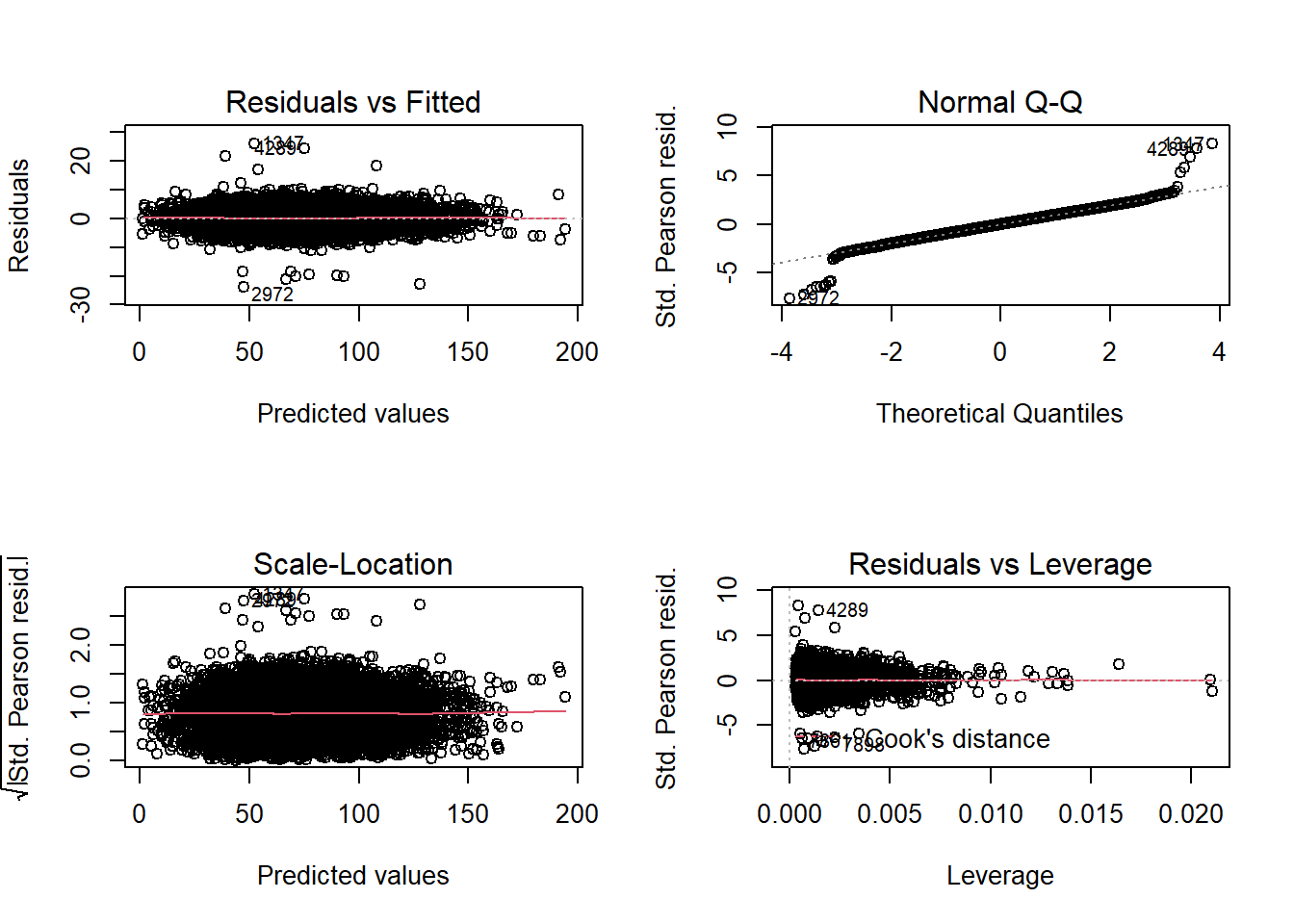
The residuals vs fitted plot shows a nice linear constant distribution of residuals. If the variance increased (fanned out) we would have heteroscedasticity, and if there’s curvature then our model is most likely missing a squared (or nonlinear) term.
Outlier Detection
The QQ plot is quite nice, majority of the points fall on the dashed line, with the exception of a few outliers, which we will now remove. Using Cook’s Distance, we can see how individual observations effect the model and will remove the points that have the biggest effect. The bigger the value, the more influence that point has on the model.
par(mfrow=c(1,1))
plot(cooks.distance(glm1))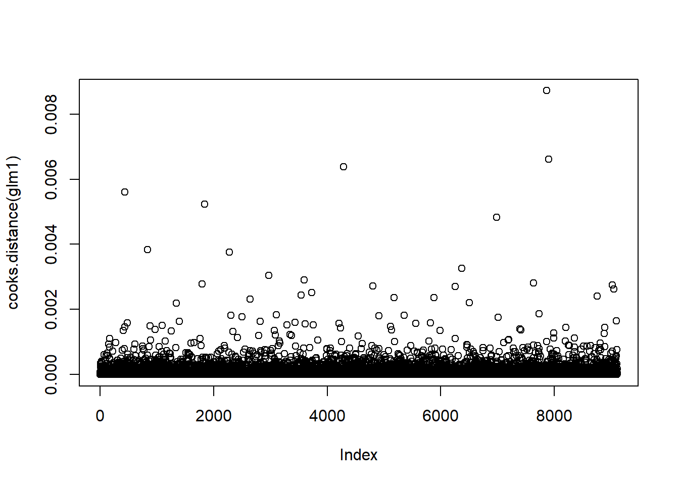
There appears to be some outliers in the dataset, we can remove about 30 data points (30/9000 or 0.3% of points). We are going to rerun the model with these outliers removed.
afltables_2019_fp_out_rem <- afltables_2019_fp %>%
  mutate(
    id = row_number(),
    cooks_d = cooks.distance(glm1)
  ) %>%
  arrange(-cooks_d) %>% # assign each obs its Cooks D
  slice(-(1:30)) %>%    # remove the top 30
  arrange(id)

# rerun the model without outliers
glm2 <- glm(
  formula = formula,
  data = afltables_2019_fp_out_rem,
  family = gaussian(link = 'identity')
)

summary(glm2)
##
## Call:
## glm(formula = formula, family = gaussian(link = "identity"),
## data = afltables_2019_fp_out_rem)
##
## Deviance Residuals:
## Min 1Q Median 3Q Max
## -18.3848 -2.0720 0.0121 2.0219 16.8099
##
## Coefficients:
## Estimate Std. Error t value Pr(>|t|)
## (Intercept) 2.069185 0.106339 19.458 <2e-16 ***
## kicks 3.014910 0.009671 311.741 <2e-16 ***
## handballs 1.987187 0.008196 242.472 <2e-16 ***
## marks 2.983426 0.015866 188.044 <2e-16 ***
## tackles 4.033991 0.015660 257.604 <2e-16 ***
## inside_50_s -0.054049 0.021004 -2.573 0.0101 *
## bounces 0.055426 0.045887 1.208 0.2271
## frees_for 1.000116 0.033831 29.562 <2e-16 ***
## frees_against -3.040852 0.032581 -93.331 <2e-16 ***
## one_percenters 0.007380 0.014268 0.517 0.6050
## hit_outs 0.996866 0.004812 207.166 <2e-16 ***
## goals 6.077538 0.036991 164.296 <2e-16 ***
## behinds 0.975389 0.047510 20.530 <2e-16 ***
## goal_assists -0.009567 0.051917 -0.184 0.8538
## ---
## Signif. codes: 0 '***' 0.001 '**' 0.01 '*' 0.05 '.' 0.1 ' ' 1
##
## (Dispersion parameter for gaussian family taken to be 9.103323)
##
## Null deviance: 6491380 on 9077 degrees of freedom
## Residual deviance: 82513 on 9064 degrees of freedom
## AIC: 45828
##
## Number of Fisher Scoring iterations: 2par(mfrow=c(2,2))
plot(glm2)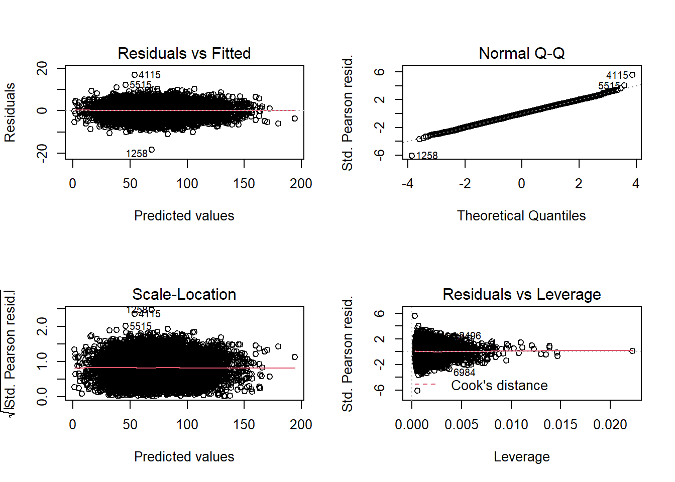
QQ plot tails are nicer.
par(mfrow=c(1,1))
plot(cooks.distance(glm2))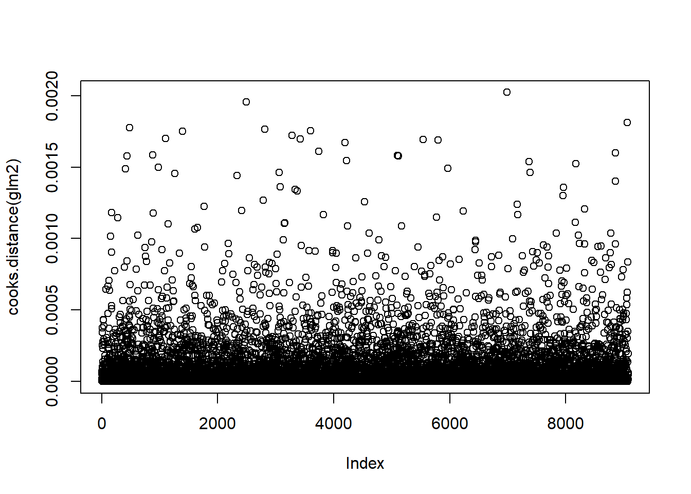
No individual points really stand out, no more outliers we can confidently remove.
Remove Non-informative Variables
The next step is to remove variables that have no predictive power on the model, and we can calculate this using the AIC metric. Akaike’s Information Criterion (AIC) is a penalisation term for models. Essentially, lower AIC is better, and we can use the following code to perform this automatically. The process may look a lot is going on, but I’ll do my best to break it down.
glm2_step <- MASS::stepAIC(glm2, direction = 'both')## Start: AIC=45828.27
## fp ~ kicks + handballs + marks + tackles + inside_50_s + bounces +
## frees_for + frees_against + one_percenters + hit_outs + goals +
## behinds + goal_assists
##
## Df Deviance AIC
## - goal_assists 1 82513 45826
## - one_percenters 1 82515 45827
## - bounces 1 82526 45828
## <none> 82513 45828
## - inside_50_s 1 82573 45833
## - behinds 1 86350 46239
## - frees_for 1 90468 46662
## - frees_against 1 161809 51940
## - goals 1 328241 58361
## - marks 1 404412 60256
## - hit_outs 1 473206 61682
## - handballs 1 617719 64101
## - tackles 1 686607 65061
## - kicks 1 967196 68171
##
## Step: AIC=45826.3
## fp ~ kicks + handballs + marks + tackles + inside_50_s + bounces +
## frees_for + frees_against + one_percenters + hit_outs + goals +
## behinds
##
## Df Deviance AIC
## - one_percenters 1 82515 45825
## - bounces 1 82526 45826
## <none> 82513 45826
## + goal_assists 1 82513 45828
## - inside_50_s 1 82579 45832
## - behinds 1 86353 46237
## - frees_for 1 90473 46660
## - frees_against 1 161814 51938
## - goals 1 330714 58427
## - marks 1 404981 60266
## - hit_outs 1 473494 61685
## - handballs 1 619111 64119
## - tackles 1 686793 65061
## - kicks 1 970731 68202
##
## Step: AIC=45824.58
## fp ~ kicks + handballs + marks + tackles + inside_50_s + bounces +
## frees_for + frees_against + hit_outs + goals + behinds
##
## Df Deviance AIC
## - bounces 1 82528 45824
## <none> 82515 45825
## + one_percenters 1 82513 45826
## + goal_assists 1 82515 45827
## - inside_50_s 1 82588 45831
## - behinds 1 86395 46240
## - frees_for 1 90519 46663
## - frees_against 1 161887 51940
## - goals 1 338089 58626
## - marks 1 412895 60440
## - hit_outs 1 477291 61756
## - handballs 1 628707 64257
## - tackles 1 687665 65071
## - kicks 1 970732 68200
##
## Step: AIC=45824
## fp ~ kicks + handballs + marks + tackles + inside_50_s + frees_for +
## frees_against + hit_outs + goals + behinds
##
## Df Deviance AIC
## <none> 82528 45824
## + bounces 1 82515 45825
## + one_percenters 1 82526 45826
## + goal_assists 1 82528 45826
## - inside_50_s 1 82598 45830
## - behinds 1 86403 46239
## - frees_for 1 90520 46661
## - frees_against 1 161972 51943
## - goals 1 338123 58624
## - marks 1 413917 60461
## - hit_outs 1 477681 61761
## - handballs 1 629399 64265
## - tackles 1 689561 65094
## - kicks 1 991022 68386We start off with AIC = 45828.27, and the stepwise AIC calculates that removing goal_assists reduces the AIC, and the new model has an AIC = 45826.3, thus improving the model. This process is repeated until removing variables no longer decreases the AIC. Using direction = 'both' allows for the algorithm to check if re-adding previously removed variables increases the AIC. In this case, it doesn’t.
Let’s check out the summary for our new model.
summary(glm2_step)##
## Call:
## glm(formula = fp ~ kicks + handballs + marks + tackles + inside_50_s +
## frees_for + frees_against + hit_outs + goals + behinds, family = gaussian(link = "identity"),
## data = afltables_2019_fp_out_rem)
##
## Deviance Residuals:
## Min 1Q Median 3Q Max
## -18.3897 -2.0712 0.0067 2.0277 16.7968
##
## Coefficients:
## Estimate Std. Error t value Pr(>|t|)
## (Intercept) 2.093698 0.096962 21.593 < 2e-16 ***
## kicks 3.016683 0.009549 315.930 < 2e-16 ***
## handballs 1.986821 0.008106 245.117 < 2e-16 ***
## marks 2.983426 0.015636 190.809 < 2e-16 ***
## tackles 4.032478 0.015615 258.248 < 2e-16 ***
## inside_50_s -0.055593 0.020097 -2.766 0.00568 **
## frees_for 0.999574 0.033735 29.630 < 2e-16 ***
## frees_against -3.041033 0.032551 -93.424 < 2e-16 ***
## hit_outs 0.996921 0.004785 208.359 < 2e-16 ***
## goals 6.073662 0.036245 167.574 < 2e-16 ***
## behinds 0.971072 0.047064 20.633 < 2e-16 ***
## ---
## Signif. codes: 0 '***' 0.001 '**' 0.01 '*' 0.05 '.' 0.1 ' ' 1
##
## (Dispersion parameter for gaussian family taken to be 9.102053)
##
## Null deviance: 6491380 on 9077 degrees of freedom
## Residual deviance: 82528 on 9067 degrees of freedom
## AIC: 45824
##
## Number of Fisher Scoring iterations: 2The model suggests that inside_50_s is a statistically significant variable, but on closer inspection it seems something weird is going on. Each inside 50 adds -0.056 (95%CI[-0.095,-0.017]) to the FP score, which begs the question: does FP penalise for inside 50’s? Using our intuition it seems much more likely that the true effect is 0, and can reasonably argued for it to be excluded from the model.
formula_3 <- "fp ~ kicks + handballs + marks + tackles + frees_for +
frees_against + hit_outs + goals + behinds"

glm3 <- glm(
  formula = formula_3,
  data = afltables_2019_fp_out_rem,
  family = gaussian(link = 'identity')
)

summary(glm3)
##
## Call:
## glm(formula = formula_3, family = gaussian(link = "identity"),
## data = afltables_2019_fp_out_rem)
##
## Deviance Residuals:
## Min 1Q Median 3Q Max
## -18.4164 -2.0786 0.0108 2.0108 16.8300
##
## Coefficients:
## Estimate Std. Error t value Pr(>|t|)
## (Intercept) 2.107037 0.096878 21.75 <2e-16 ***
## kicks 3.004733 0.008519 352.72 <2e-16 ***
## handballs 1.982782 0.007976 248.59 <2e-16 ***
## marks 2.991265 0.015382 194.46 <2e-16 ***
## tackles 4.027332 0.015509 259.67 <2e-16 ***
## frees_for 1.000197 0.033746 29.64 <2e-16 ***
## frees_against -3.043979 0.032545 -93.53 <2e-16 ***
## hit_outs 0.996308 0.004781 208.38 <2e-16 ***
## goals 6.062463 0.036031 168.26 <2e-16 ***
## behinds 0.953944 0.046672 20.44 <2e-16 ***
## ---
## Signif. codes: 0 '***' 0.001 '**' 0.01 '*' 0.05 '.' 0.1 ' ' 1
##
## (Dispersion parameter for gaussian family taken to be 9.10873)
##
## Null deviance: 6491380 on 9077 degrees of freedom
## Residual deviance: 82598 on 9068 degrees of freedom
## AIC: 45830
##
## Number of Fisher Scoring iterations: 2Interestingly, the AIC did increase but the residual deviance decreased.
Presenting Results
Next step is to convey the estimates and confidence intervals.
library(broom)
glm3_coef <- tidy(glm3)
glm3_confint <- glm3_coef %>%
  mutate(
    lb = estimate-1.96*std.error,
    ub = estimate+1.96*std.error,
  )

library(ggplot2)
ggplot(glm3_confint, aes(x=estimate, y=reorder(term, desc(term)))) +
  geom_errorbar(aes(xmin=lb, xmax=ub), width=.3) +
  geom_point() +
  ggtitle("The Effect of AFL Statistics on Total Fantasy Points") +
  xlab("Estimate (95% CI)") + ylab("Term")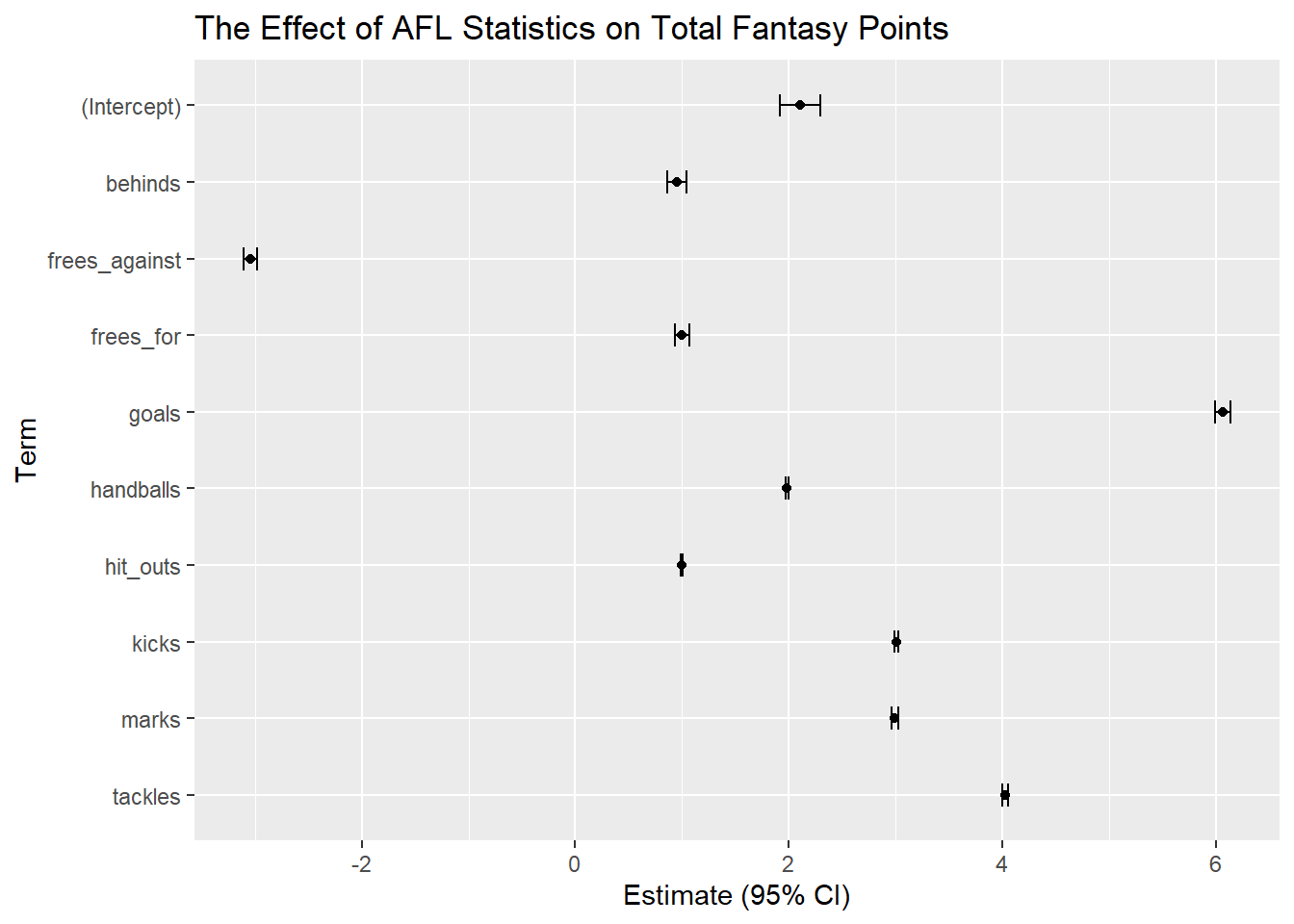
We are 95% confident that the true mean of the term is between these confidence intervals.
glm3_confint_clean <-
  glm3_confint %>%
  mutate(
    estimate = round(estimate, 2),
    lb = round(lb, 2),
    ub = round(ub, 2)
  ) %>%
  select(Term = term, Estimate = estimate, `Lower Bound` = lb, `Upper Bound` = ub)

DT::datatable(glm3_confint_clean, rownames = F, width = 500,
              caption = "The Effect of AFL Statistics on Total Fantasy Points (95%CI)",
              options = list(dom = 't'))
Conclusion
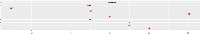
It turns out that Fantasy Points have been made publicly available, which means we can now compare our results to the real deal. (I’ve applied a shift of 2, mainly to illustrate the use of (Intercept) in the model).
glm3_confint_true <- glm3_confint %>%
  mutate(
    true_estimate = case_when(
      term == "kicks" ~ 3,
      term == "handballs" ~ 2,
      term == "marks" ~ 3,
      term == "tackles" ~ 4,
      term == "frees_for" ~ 1,
      term == "frees_against" ~ -3,
      term == "hit_outs" ~ 1,
      term == "goals" ~ 6,
      term == "behinds" ~ 1
    )
  )

ggplot(glm3_confint_true, aes(x=estimate, y=reorder(term, desc(term)))) +
  geom_errorbar(aes(xmin=lb, xmax=ub), width=.3) +
  geom_point() +
  geom_point(aes(x=true_estimate, y=reorder(term, desc(term))), colour = 'red') +
  ggtitle("The Effect of AFL Statistics on Total Fantasy Points") +
  xlab("Estimate (95% CI)") + ylab("Term")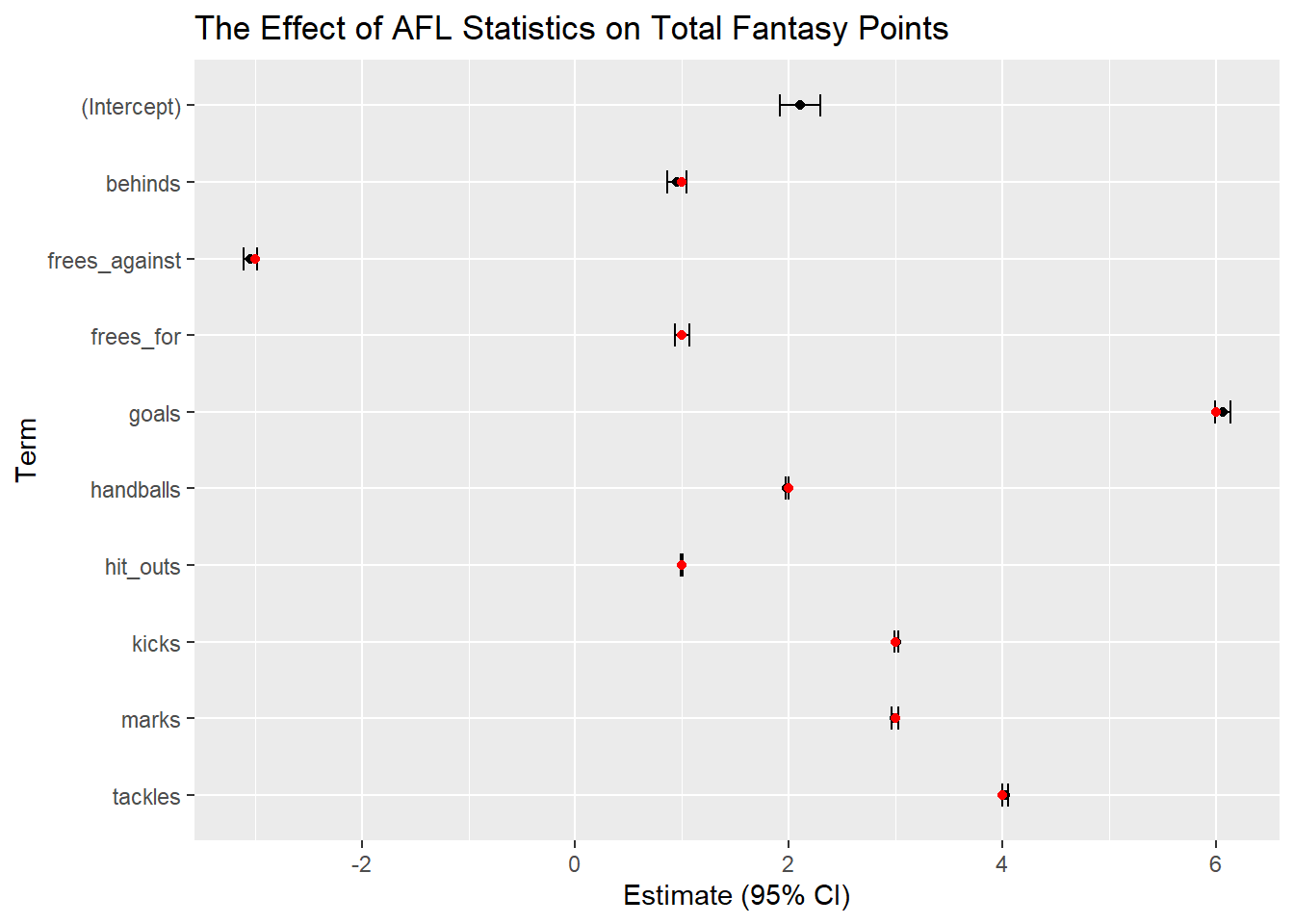
The red dots represent the true points assigned to each statistic, and we can see that after this process our model correctly identifies the true values, despite the addition of random noise and artificial outliers.
Make sure to tweet at me @crow_data_sci about ideas, corrections and clarifications! I’m also planning to do a Bayesian/simulation based regression in brms, that will follow the same data and flow.